Learning Lane-Structured Conditioning Fields for Online HD Mapping

Andrea Bertogalli; Anthony Dell'Eva; Marcello Ceresini; Federico Pirazzoli; Filippo D'Addeo; Lorenzo Cipelli; Nicola Marinello; Massimo Bertozzi

Abstract

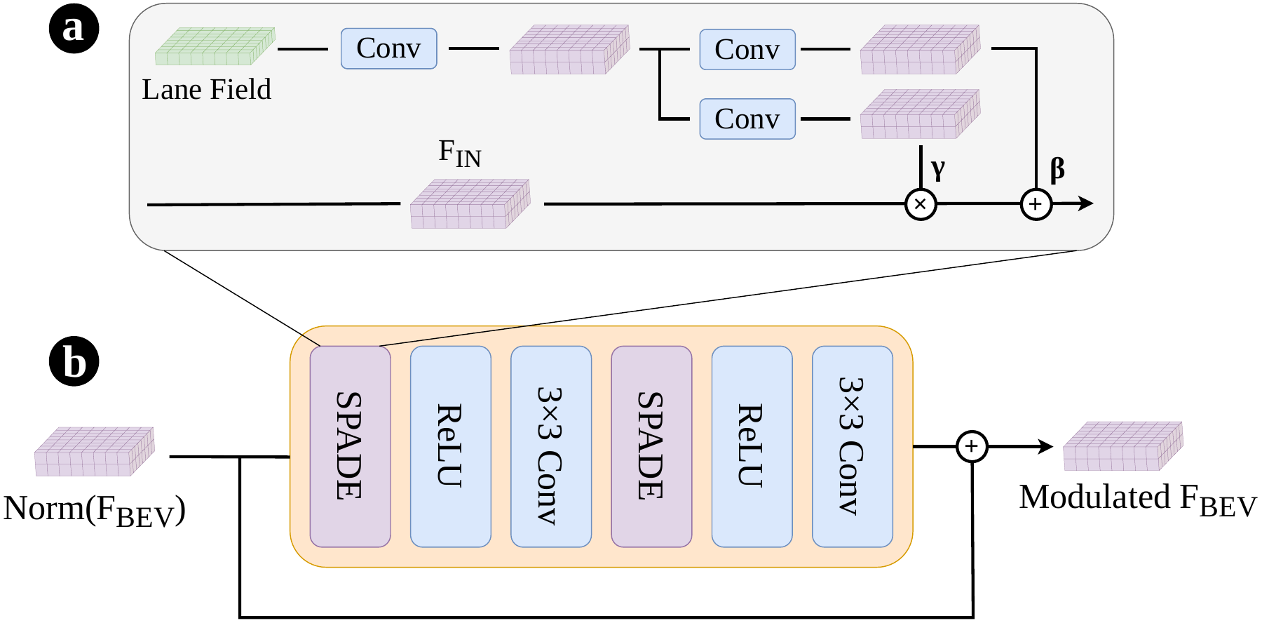
High-definition maps provide critical structural information for downstream autonomous driving tasks. Recent methods increasingly rely on external priors to improve prediction accuracy and robustness. Yet, existing prior representations expose a trade-off: dense rasters are easy to integrate but ignore certain map geometric properties, while sparse vectors preserve geometric structure but require dedicated encoders and are difficult to plug into existing architectures. Moreover, external priors can be inaccurate, costly to acquire, or difficult to maintain, motivating a structural representation that can provide geometric guidance while remaining learnable and broadly applicable. We address this limitation with the Lane Field, a dense BEV-aligned geometric representation that encodes local lane structure at each spatial location and can be either predicted from onboard observations or constructed from external map priors. Building on this representation, we introduce a plug-and-play framework that enhances online HD mapping through two complementary mechanisms: BEV feature modulation, which injects lane-structured cues into latent BEV features, and deformable attention guidance, which steers query sampling toward the underlying lane geometry. We primarily evaluate our method on OpenLane-V2, showing that conditioning BEV features and guiding deformable attention with local lane geometry enables our framework to consistently improve existing methods and achieve state-of-the-art performance on lane segment perception.

Overview

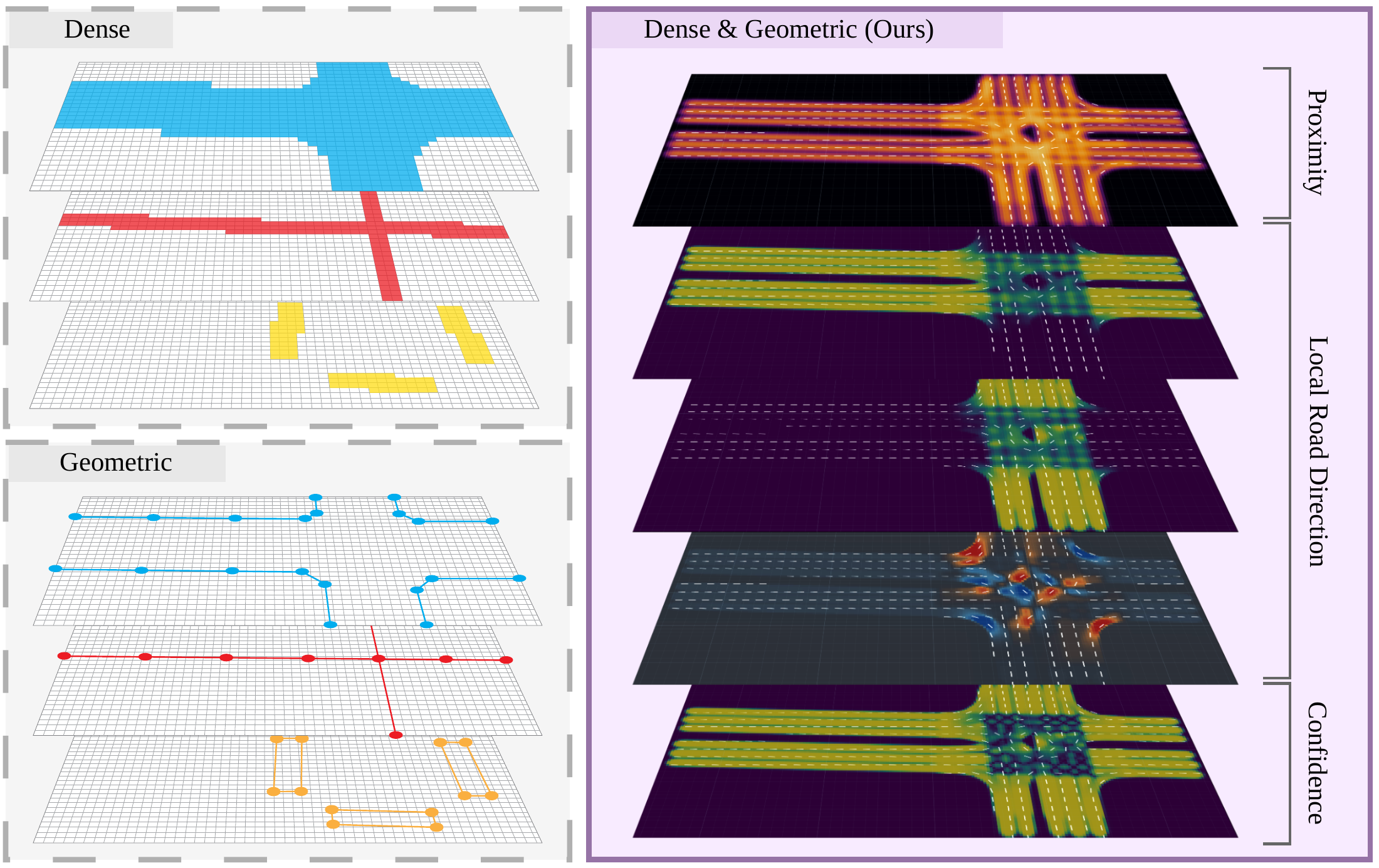
A dense field for proximity, orientation and confidence. Lane Field turns local lane geometry into a conditioning signal for BEV features and deformable attention.

Comparison of a dense raster map, sparse vector geometry, and the Lane Field channels for proximity, local direction, and confidence. — **Figure 1.** Lane Field combines the geometric meaning of vectorized maps with a dense, BEV-aligned spatial structure.

Video 1. Online HD map reconstruction on OpenLane-V2. Surround-view camera observations are shown alongside the predicted Lane Field and vectorized map geometry.

0:59 · No audioDownload video

Method

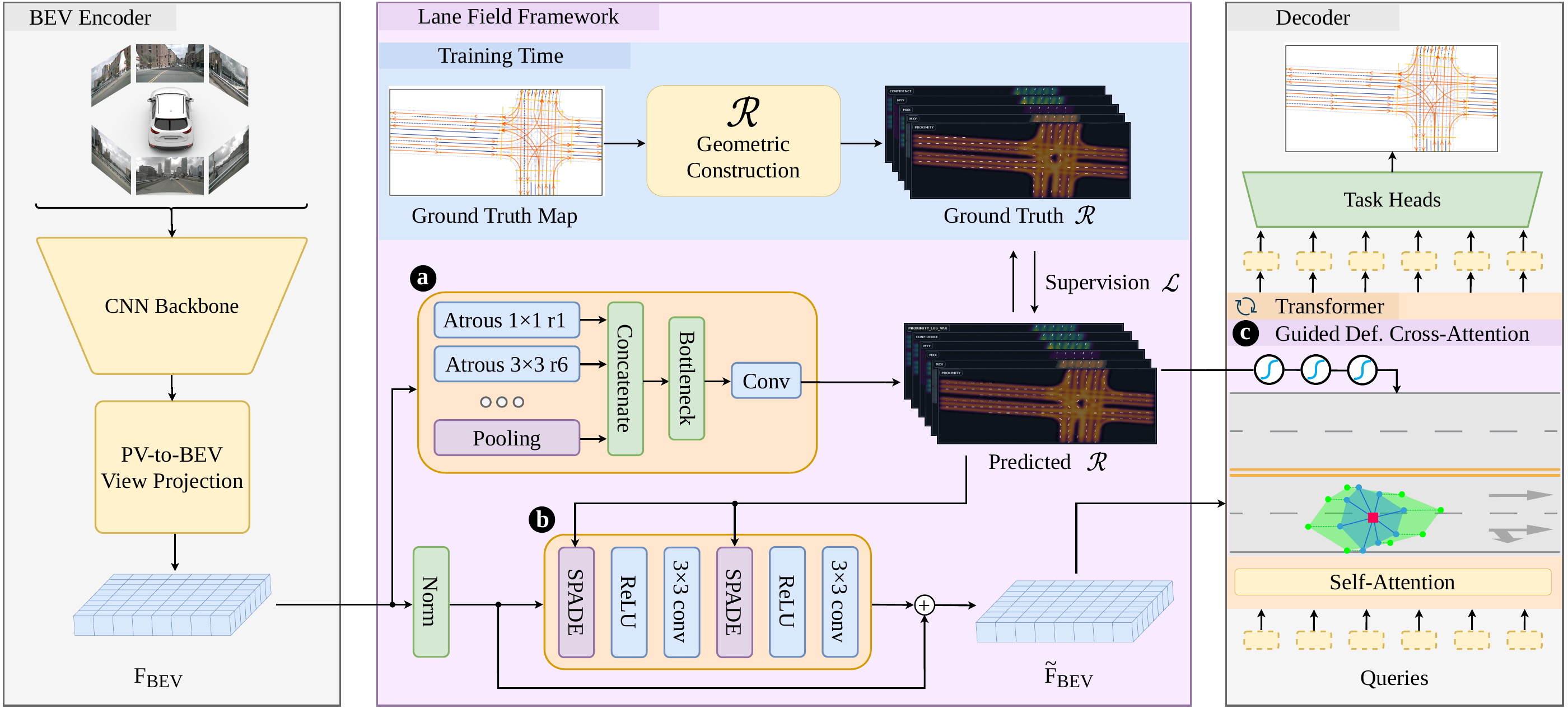
Camera observations → BEV features → Lane Field prediction → feature modulation and guided attention. Vector annotations provide analytic supervision during training; external map priors can supply the same representation.

Camera observations are encoded into BEV features. A prediction head estimates the Lane Field, which modulates BEV features and guides deformable attention in the decoder. — **Figure 2.** Overview of the framework: (a) Lane Field prediction, supervised with fields constructed from vector annotations; (b) BEV feature modulation; (c) guided deformable attention.

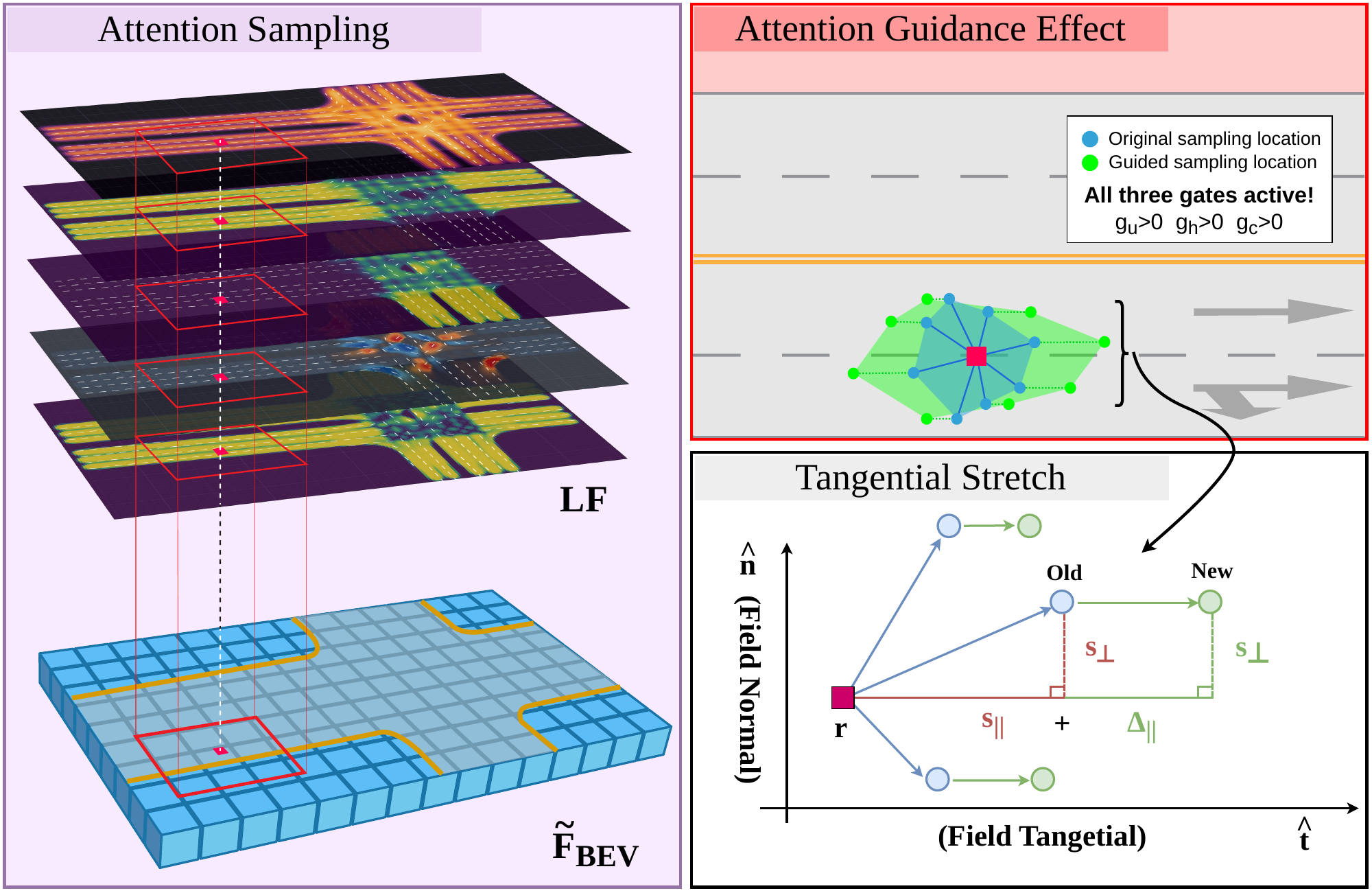
Inside the framework BEV modulation & attention guidance

SPADE-like modulation predicts spatially varying gamma and beta parameters from the Lane Field and applies them inside a residual BEV refinement block. — **Figure 3. BEV feature modulation.** The Lane Field predicts spatially varying affine parameters γ and β. A residual block uses these parameters to refine the BEV features.

Lane Field guided attention preserves the normal offset and stretches the tangential offset along the local lane direction when the three guidance gates are active. — **Figure 4. Deformable attention guidance.** Sampling offsets stretch along the lane direction. Directional confidence, uncertainty, and a learnable per-head gate control the strength of the guidance.

Lane Field prediction

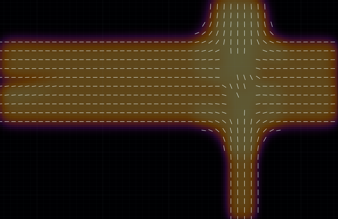
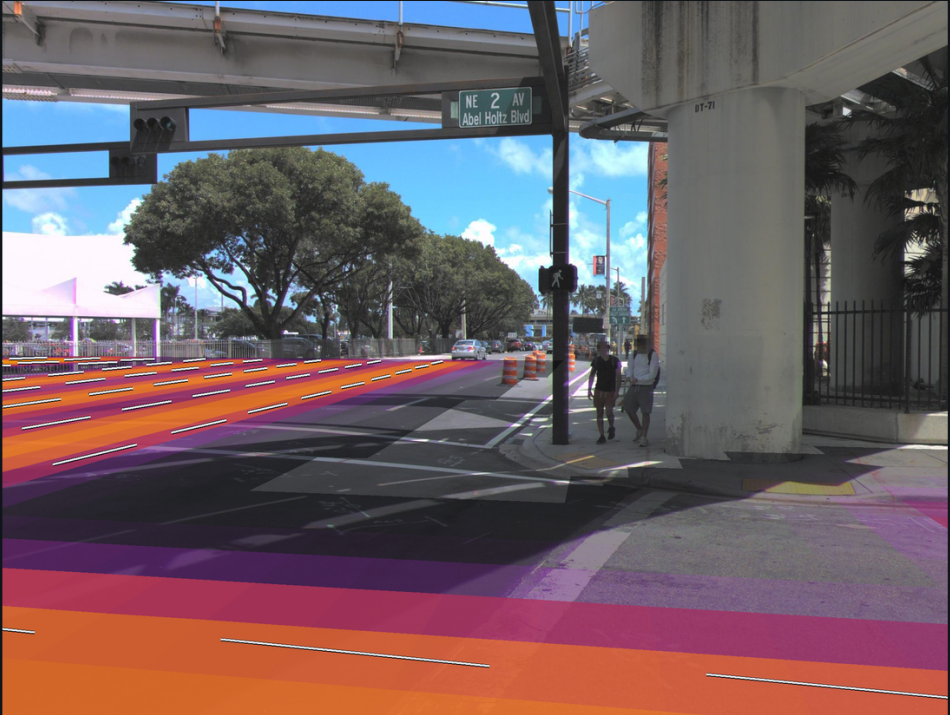
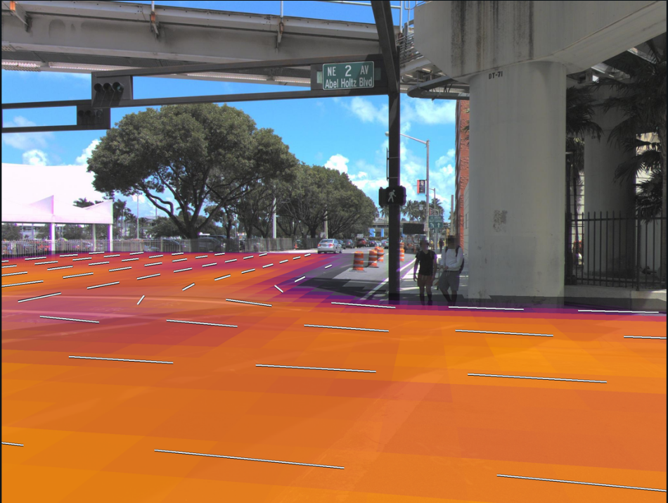
The representation describes proximity, local lane direction, and directional confidence across the BEV grid. The following video shows predicted fields across driving scenes.

Video 2. Lane Field predictions across driving scenes. The visualizations show dense geometric structure in relation to image observations and the local road map.

3:56 · No audioDownload video

Visualizations

Build the representation interactively, then inspect the paper’s maps, attention patterns and uncertainty estimates. Select any research figure to enlarge it.

From lane geometry to a dense field

The Lane Field is constructed analytically from vector map annotations. Each lane segment contributes both a smooth spatial weight and an unoriented direction to every location p in the bird’s-eye-view grid.

Interactive construction

Build the field, one point at a time.

Analytic demo

Straight road Bend Crossing

p = (2.0, 2.0) m

Drag p, any segment or its endpoints A and B. In Integrate, drag q(t) too.

Angle θ 0°

Length ℓ 20.0 m

Arrow keys: point p · Tab switches target

Segments & lane boundaries

Start with a centerline.

Split the lane into finite segments. Each has endpoints A_i, B_i and a unit tangent t̂_i. The point p is one cell of the BEV grid.

{\hat{t}}_{i} = \frac{B_{i} - A_{i}}{ℓ_{i}}

A sparse line becomes a dense signal: every segment will contribute to every grid cell.

Select a segment on the map or above it. Drag its handles or use the angle and length sliders. Shared endpoints keep a bend connected.

R(p)Active segments · 5 channels

M_xx0

M_xy0

M_yy0

P0

C0

Illustrative geometry · σ = 1.75 m, lane width = 3.5 m. Outputs use the paper’s analytic integral and supplementary target normalization and proximity mask.

Equations & target normalization Paper §3.2 · Supplementary: derivation & implementation

1. Spread each lane segment over the grid

Split each centerline into straight segments. Segment i has endpoints A_i and B_i, length ℓ_i, unit tangent t̂_i = (B_i − A_i) / ℓ_i, and average lane width w̄_i. Its Gaussian spread is σ_i = f · w̄_i.

I_{i} (p) = ℓ_{i} \int_{0}^{1} \exp (- \frac{{‖ p - A_{i} - t (B_{i} - A_{i}) ‖}^{2}}{2 σ_{i}^{2}}) d t

Here, t moves from one endpoint to the other. Integrating the Gaussian along the finite segment gives a smooth contribution I_i(p): nearby locations receive more support, and distant locations receive less. The factor f controls how broadly that support spreads.

2. Accumulate direction and proximity

At each grid location, sum the contributions of all segments. Weighting each tangent’s outer product produces a symmetric 2 × 2 directional tensor M; summing the weights alone gives the proximity P.

M (p) = \sum_{i} I_{i} (p) {\hat{t}}_{i} {\hat{t}}_{i}^{⊤}

P (p) = \sum_{i} I_{i} (p)

The outer product is unchanged when a tangent is reversed, so the tensor describes a lane’s axis rather than its travel direction. Proximity measures how strongly nearby lane geometry supports that location.

3. Measure directional agreement

Let λ₁ ≥ λ₂ be the eigenvalues of M(p). Their relative difference defines the direction confidence C: it is high when a single axis dominates and lower when competing orientations contribute, as at an intersection.

C (p) = \frac{λ_{1} (p) - λ_{2} (p)}{λ_{1} (p) + λ_{2} (p)}

The resulting representation has five channels at each BEV location: three tensor entries, proximity, and directional confidence.

R (p) = [M_{x x} (p), M_{x y} (p), M_{y y} (p), P (p), C (p)]

The demo evaluates the closed-form integral from the supplement: I_i(p) = σ_i√(π/2) exp(−d_⊥,i² / 2σ_i²) [erf(u_1,i) − erf(u_0,i)], where a_i = (p − A_i)^⊤t̂_i, u_0,i = −a_i / (√2 σ_i) and u_1,i = (ℓ_i − a_i) / (√2 σ_i). The projection onto the supporting line is not clamped; the integration bounds account for finite endpoints.

For training targets, P^gt = P / (P + 1) and m = sigmoid(20(P^gt − 0.3)). The output tensor is M^gt = M / (tr(M) + ε) · m, and C^gt = C · m. The five live outputs above use these transformations; the matrix and eigenvalue readouts show the raw accumulations. The implementation also uses a minimum Gaussian spread and numerical stabilization. These constructed fields supervise the prediction head and can also encode external map priors.

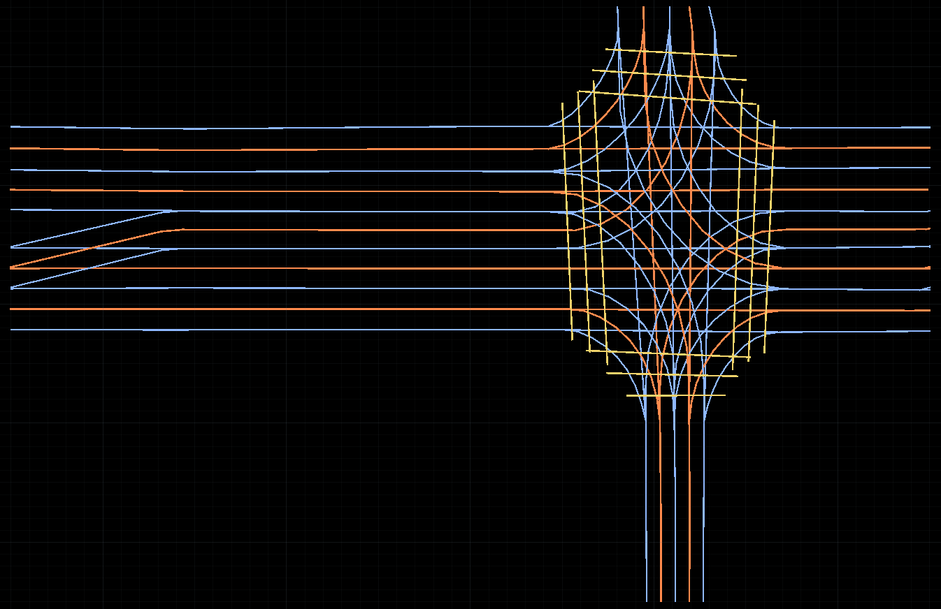
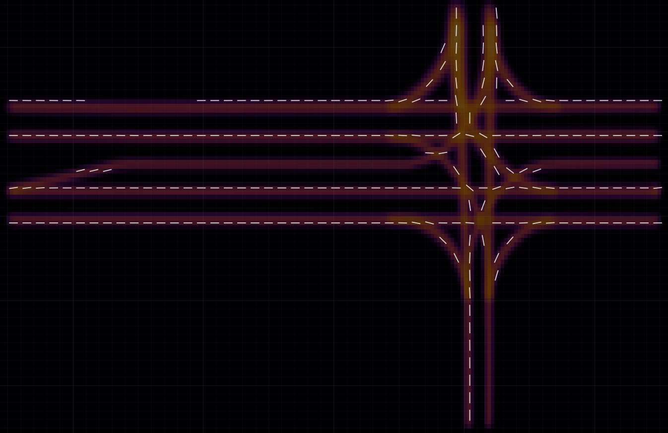
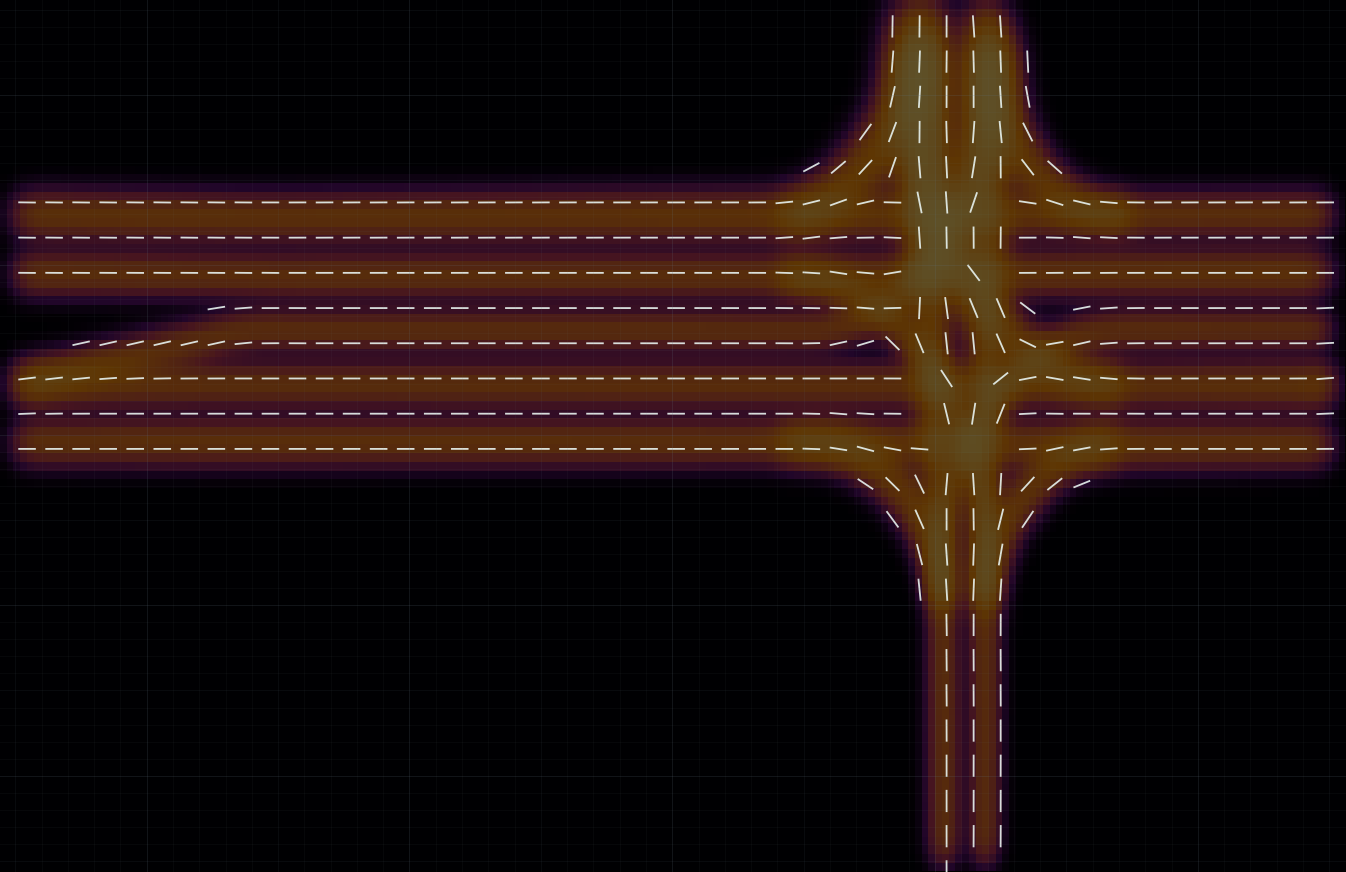
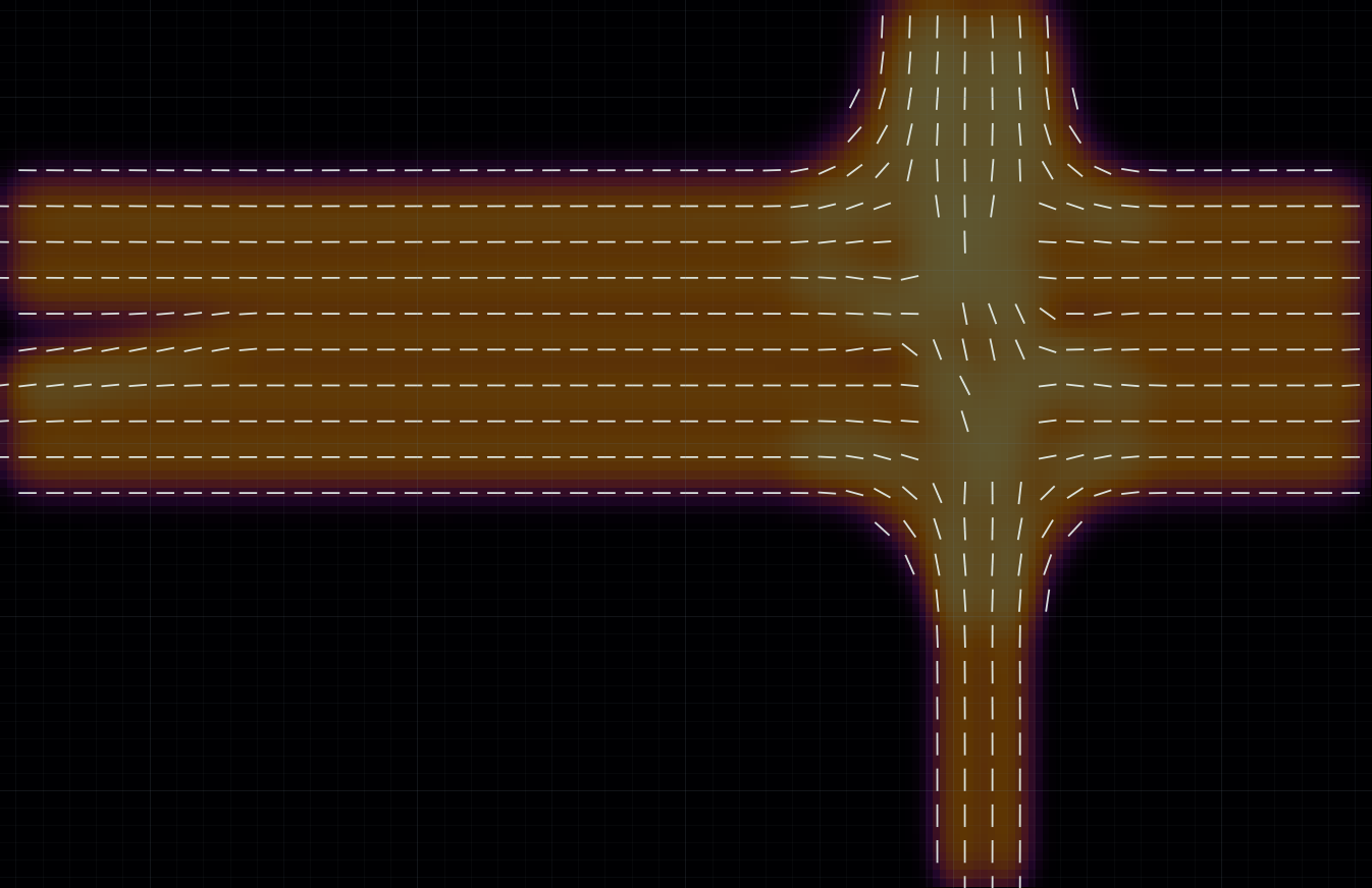
How wide should the field spread?

The demo keeps σ fixed. In the paper, σ_i = f · w̄_i adapts it to lane width. Compare the actual ground-truth fields below: increasing f broadens support. The paper uses f = 0.50.

Vector map annotations for the intersection used to construct the ground-truth Lane Field. — **f = 0.25.** Narrow, localized support around the centerlines. The Gaussian weight at the lane edge is approximately **13%**, following exp(−1 / (8f²)). These weights describe the field construction, not detection accuracy.

Ground-truth Lane Field for the same intersection with Gaussian spread factor 0.25. — **f = 0.25.** Narrow, localized support around the centerlines. The Gaussian weight at the lane edge is approximately **13%**, following exp(−1 / (8f²)). These weights describe the field construction, not detection accuracy.

Ground-truth Lane Field for the same intersection with Gaussian spread factor 0.50. — **f = 0.50.** A balance between localized support and spatial coverage. The Gaussian weight at the lane edge is approximately **61%**, following exp(−1 / (8f²)). These weights describe the field construction, not detection accuracy.

Ground-truth Lane Field for the same intersection with Gaussian spread factor 0.75. — **f = 0.75.** Broader support extends farther from the centerlines. The Gaussian weight at the lane edge is approximately **80%**, following exp(−1 / (8f²)). These weights describe the field construction, not detection accuracy.

Ground-truth Lane Field for the same intersection with Gaussian spread factor 1.00. — **f = 1.00.** The broadest support among the provided settings. The Gaussian weight at the lane edge is approximately **88%**, following exp(−1 / (8f²)). These weights describe the field construction, not detection accuracy.

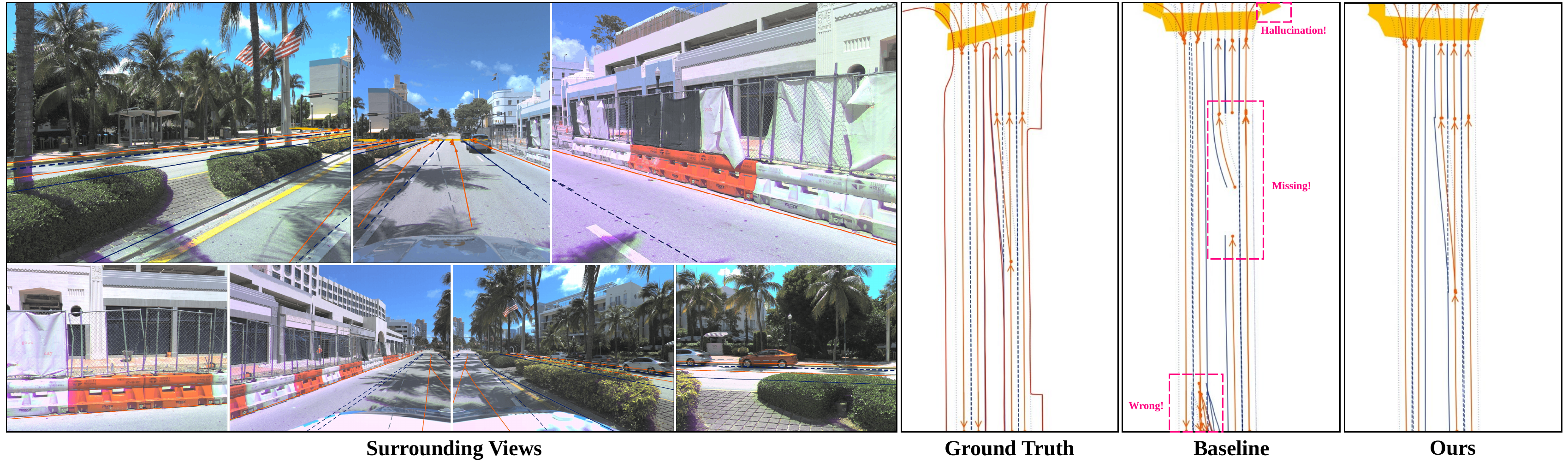
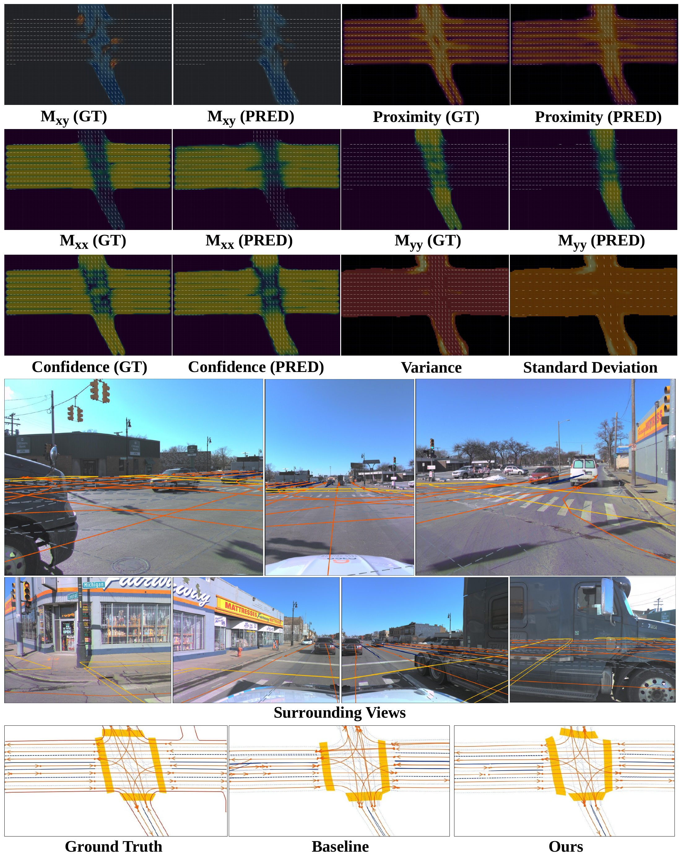
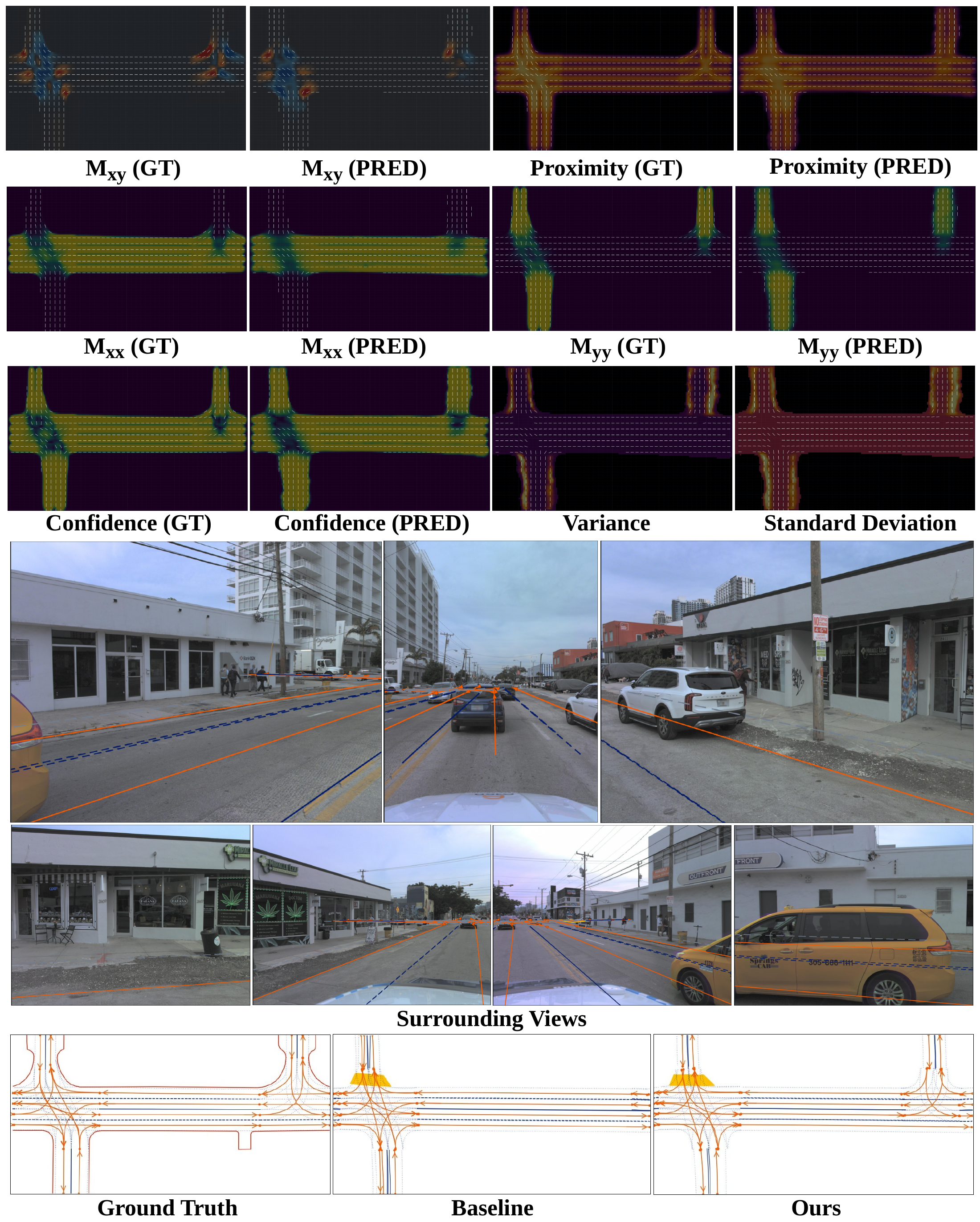
Qualitative map predictions

Surround-view camera images with reprojected map predictions, followed by ground truth, LaneSegNet baseline, and Lane Field enhanced BEV maps. Annotations mark hallucinated, missing, and incorrect baseline elements. — **Figure 5.** Predictions on OpenLane-V2. Camera-view projections and BEV comparisons show the ground truth, LaneSegNet baseline, and our enhanced variant. Lane Field helps preserve the lane layout and reduces the errors highlighted in the figure.

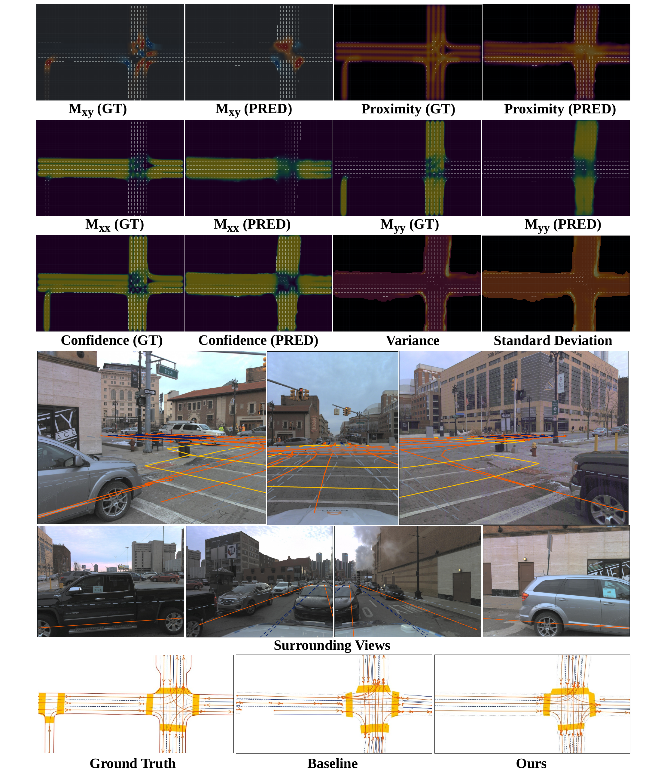
More scenes: pedestrian crossings and distant intersections

Supplementary scene with ground truth and predicted Lane Field channels, surround-view camera images, and the ground truth, baseline, and enhanced HD maps. — **Pedestrian crossing.** The baseline misses a crossing and makes inaccurate local predictions; Lane Field conditioning recovers the crossing and improves the map structure in this example.

Supplementary scene comparing Lane Field channel predictions and HD maps around a distant intersection. — **Distant intersection.** The enhanced variant preserves the intersection structure more accurately. The upper panels compare predicted and ground-truth Lane Field channels.

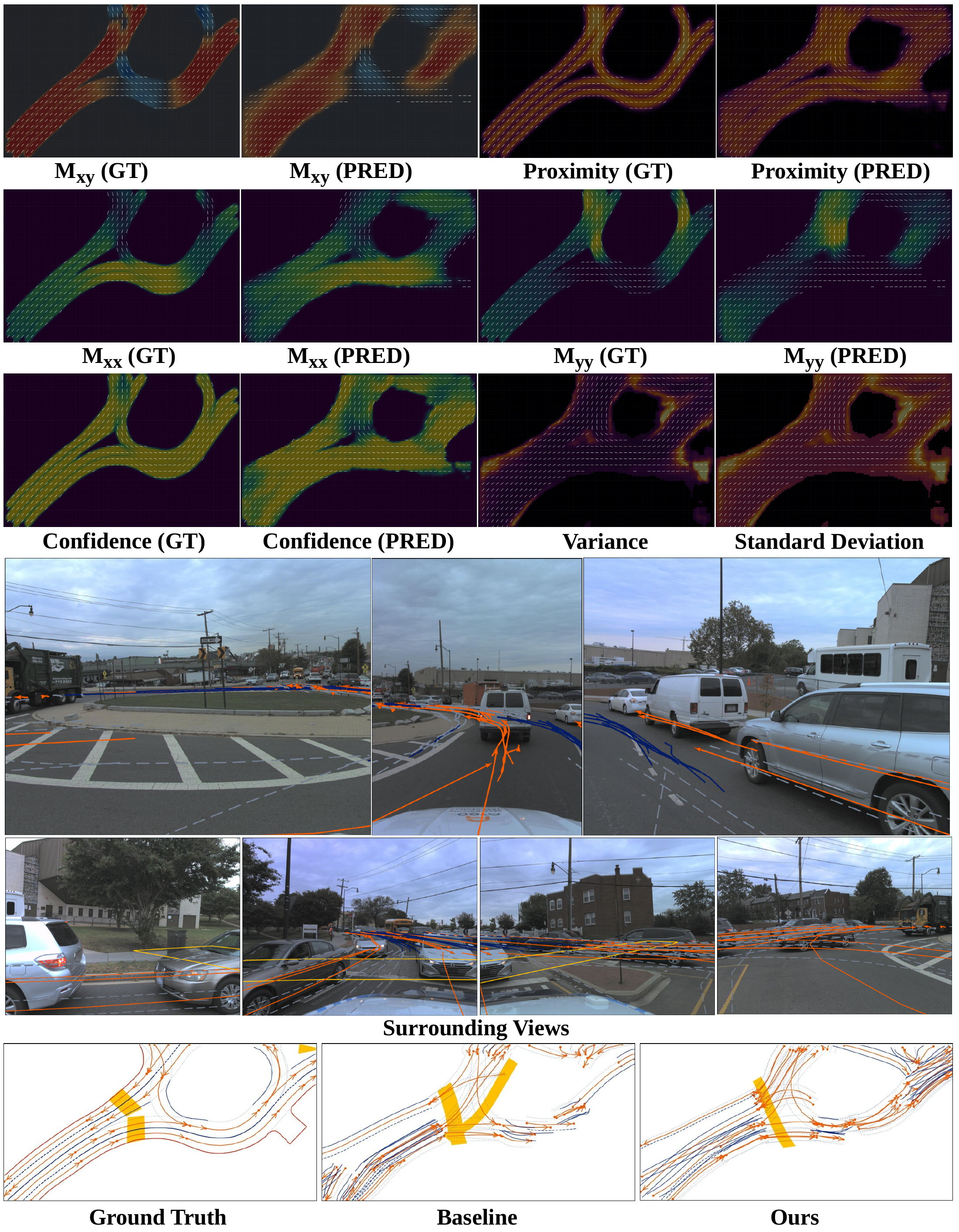
Failure cases: roundabouts and missed crossings

Roundabout example with Lane Field channels, camera views, and HD maps showing errors in both the baseline and enhanced variant. — **Roundabout.** Both methods struggle in this rare dataset scenario, although the enhanced variant shows somewhat better awareness of the overall lane structure.

Challenging scene in which the Lane Field enhanced model improves lane structure but still misses a pedestrian crossing. — **Missed crossing.** Lane Field does not explicitly encode pedestrian crossing regions, so the model can still miss crossings in challenging scenes.

Where the decoder samples

Compare the learned sampling offsets with the Lane Field guided offsets in the last decoder layer. Guidance stretches the pattern along reliable lane directions and is suppressed where the direction is ambiguous or the prediction is uncertain.

On the road: original sampling locations around the reference point. — **On the road.** At a road-supported reference point, the guided pattern stretches along the lane and its principal axis becomes better aligned with the local direction.

On the road: sampling locations after Lane Field guidance. — **On the road.** At a road-supported reference point, the guided pattern stretches along the lane and its principal axis becomes better aligned with the local direction.

At an intersection: original sampling locations around the reference point. — **At an intersection.** At the intersection, directional confidence is close to zero. The confidence gate suppresses the guidance, keeping the pattern close to the learned offsets.

At an intersection: sampling locations after Lane Field guidance. — **At an intersection.** At the intersection, directional confidence is close to zero. The confidence gate suppresses the guidance, keeping the pattern close to the learned offsets.

High uncertainty: original sampling locations around the reference point. — **High uncertainty.** High predicted variance suppresses the guidance through the uncertainty gate. Red areas in the third panel mark the regions considered reliable by that gate.

High uncertainty: sampling locations after Lane Field guidance. — **High uncertainty.** High predicted variance suppresses the guidance through the uncertainty gate. Red areas in the third panel mark the regions considered reliable by that gate.

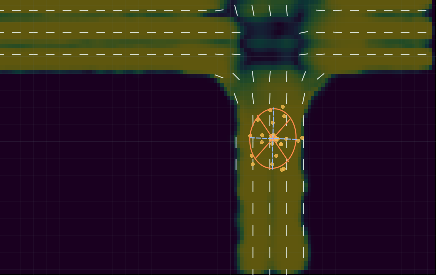
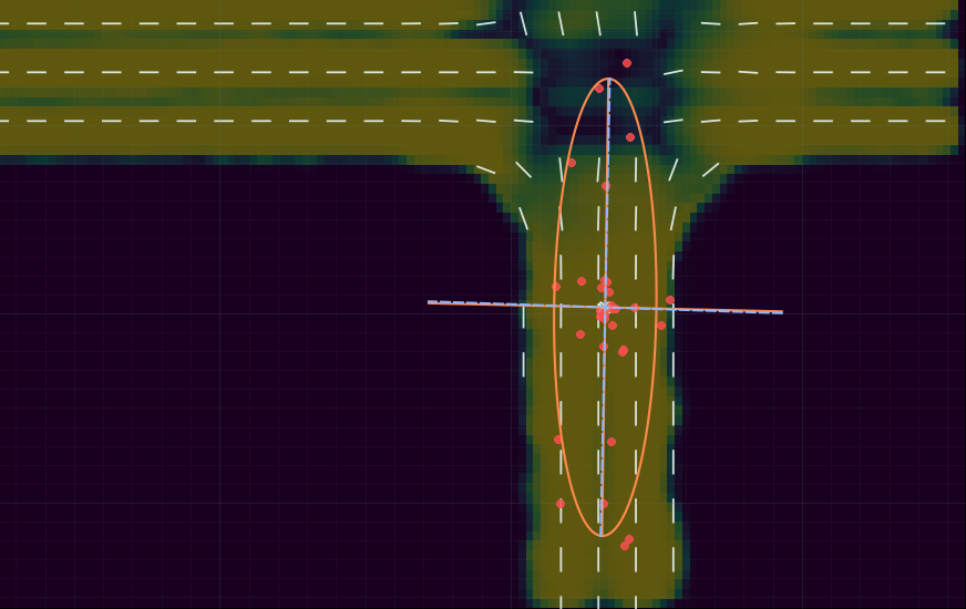
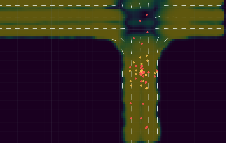
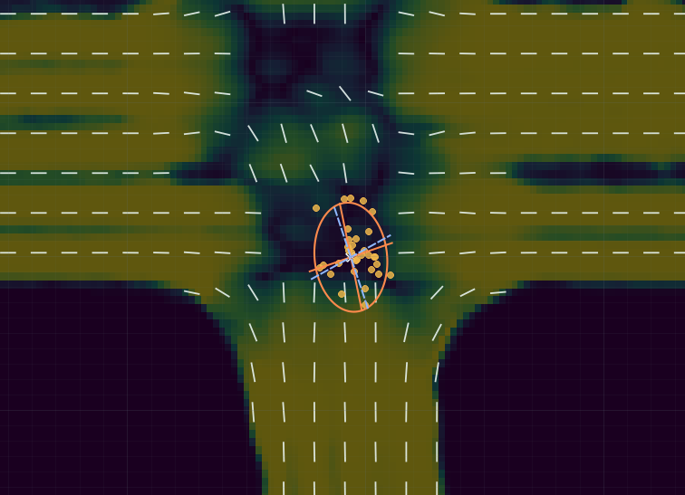
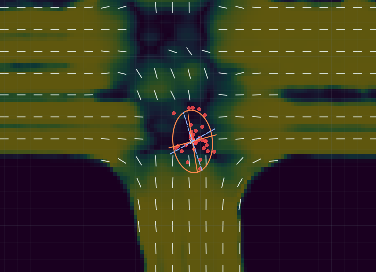
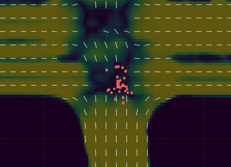
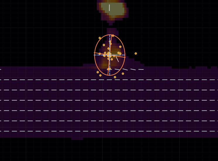
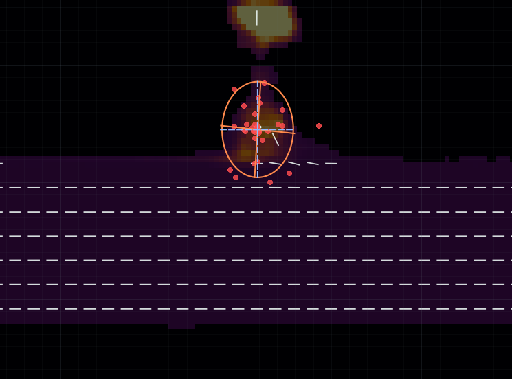
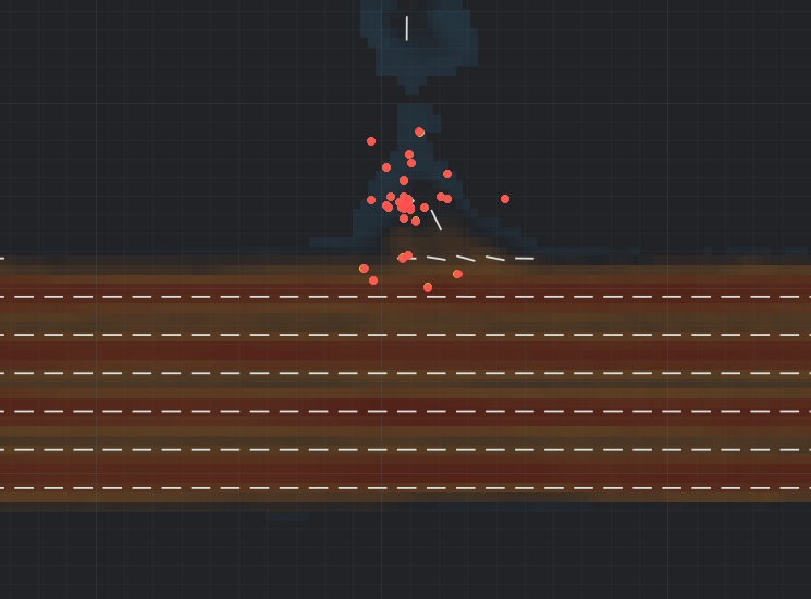
These examples use an attention head whose learned head gate converges close to one, as described in the supplementary analysis.

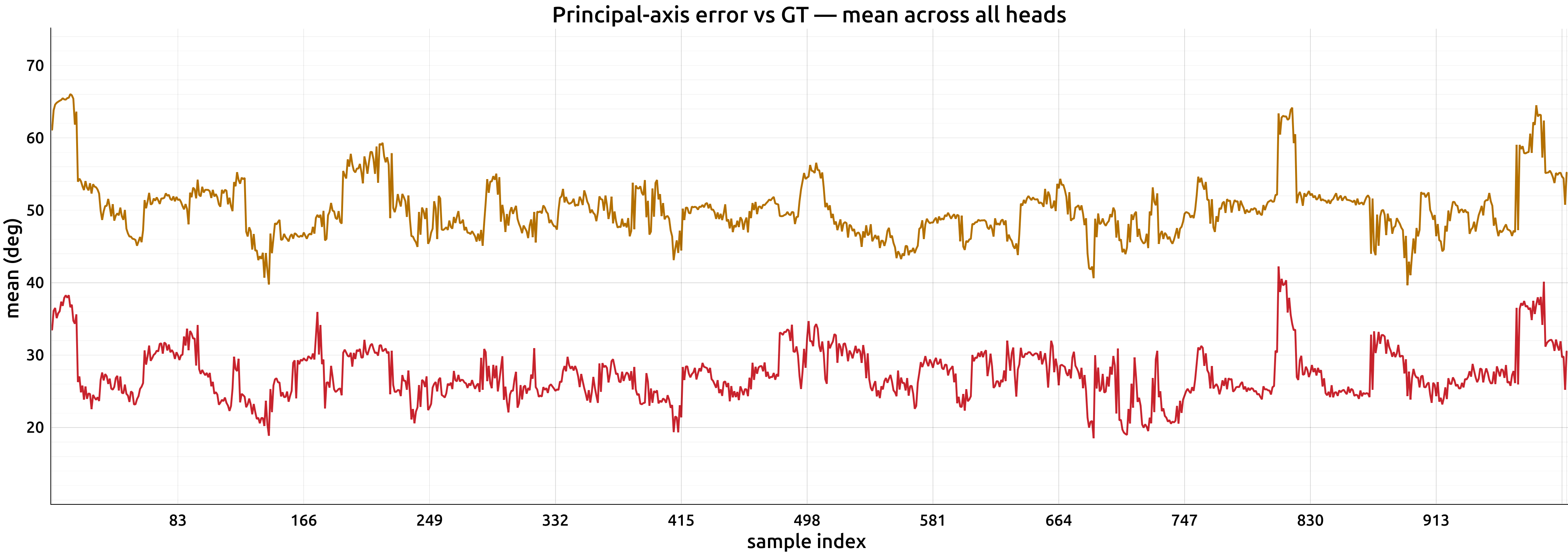
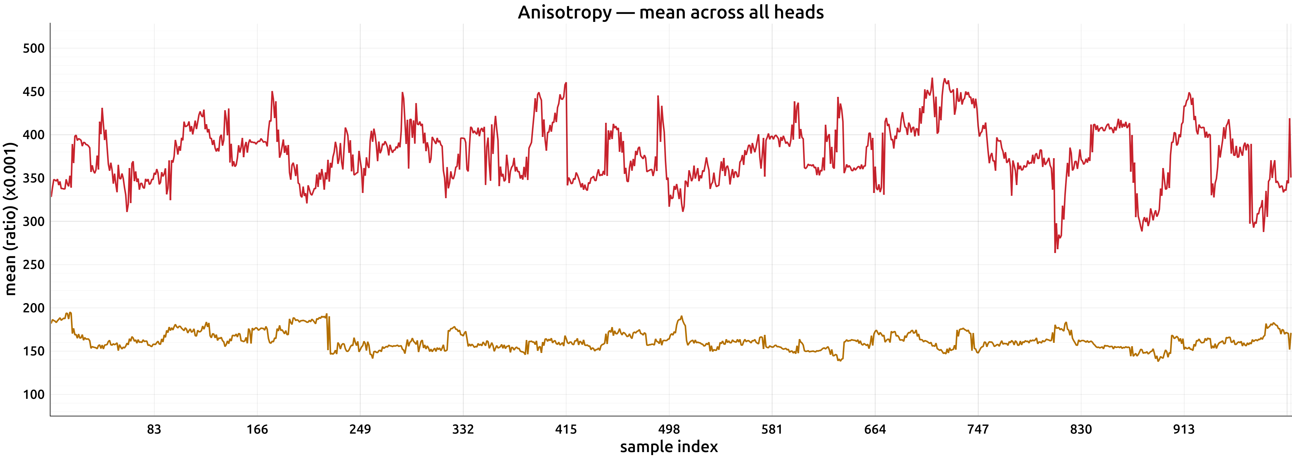
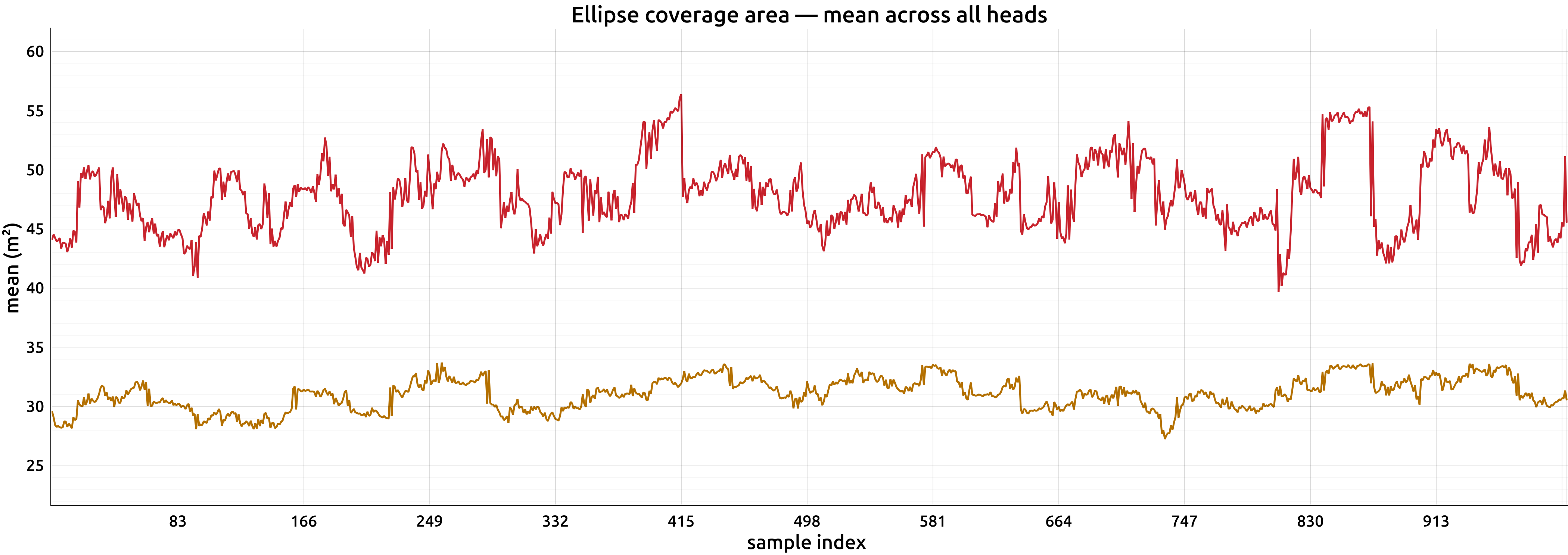
Attention measurements across 1,000 validation samples

Original Lane Attention (orange) and guided attention (red), averaged across heads. The values below are the aggregate measurements reported in the supplementary table.

Alignment error: original plot comparing original Lane Attention in orange and guided attention in red across validation samples. — **Alignment error.** Angular error between the principal sampling axis and the ground-truth lane direction. Lower is better.

Anisotropy: original plot comparing original Lane Attention in orange and guided attention in red across validation samples. — **Anisotropy.** The guided sampling pattern is more elongated along the lane direction.

Spatial coverage: original plot comparing original Lane Attention in orange and guided attention in red across validation samples. — **Spatial coverage.** Average area covered by sampling locations per reference point.

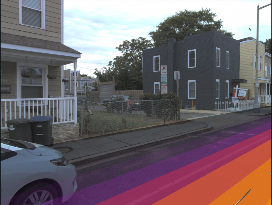
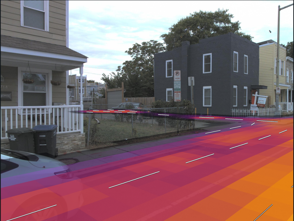
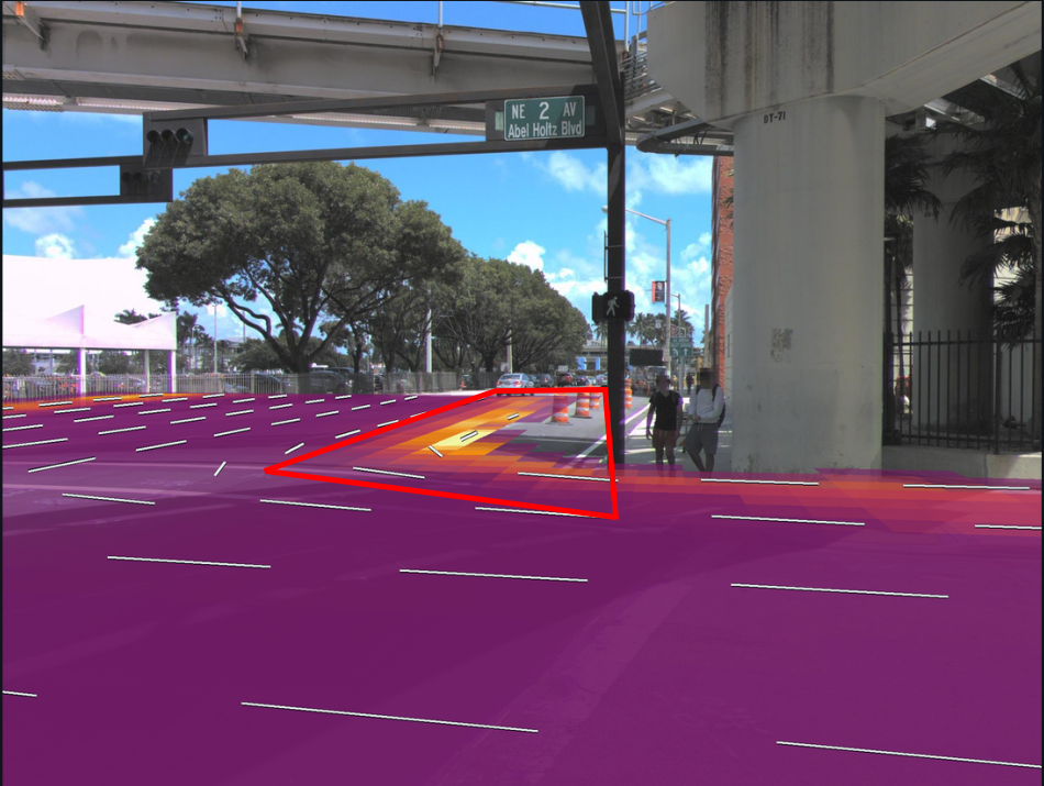
Knowing when the field is uncertain

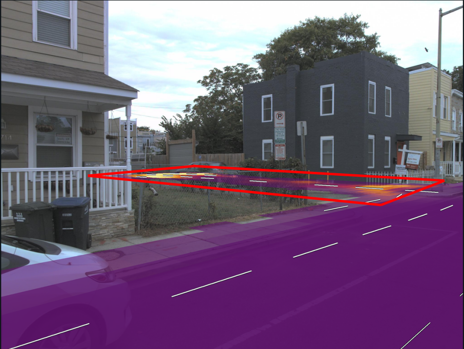
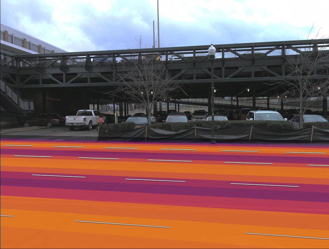
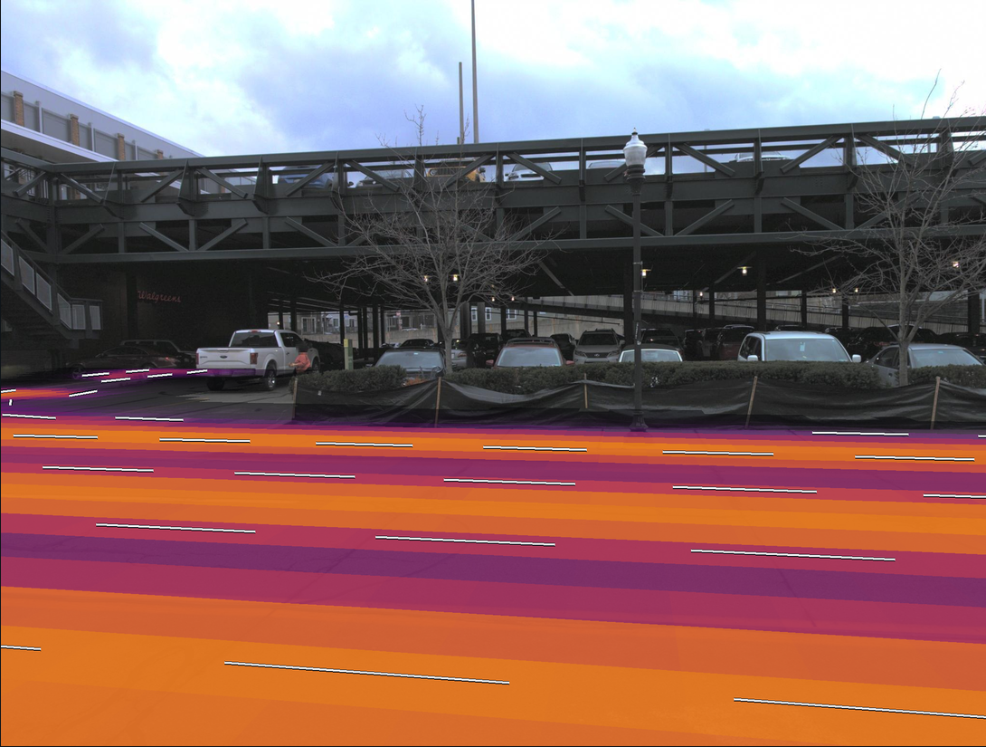
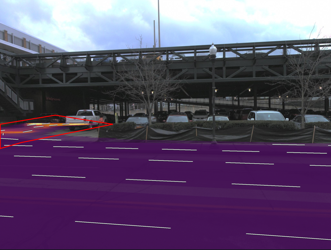
Predicted proximity can extend into regions that are not annotated as lanes. The predicted variance provides a separate reliability cue, allowing the downstream modules to reduce their reliance on uncertain geometry.

Driveway: ground-truth proximity projected onto the camera image. — **Driveway.** The driveway is not annotated in the ground truth. The model predicts both high proximity and high variance there, indicating uncertainty.

Driveway: predicted proximity projected onto the camera image. — **Driveway.** The driveway is not annotated in the ground truth. The model predicts both high proximity and high variance there, indicating uncertainty.

Parking entrance: ground-truth proximity projected onto the camera image. — **Parking entrance.** The parking entrance is unannotated. High variance accompanies the proximity prediction in that region and can reduce the strength of the guidance.

Parking entrance: predicted proximity projected onto the camera image. — **Parking entrance.** The parking entrance is unannotated. High variance accompanies the proximity prediction in that region and can reduce the strength of the guidance.

Ambiguous free space: ground-truth proximity projected onto the camera image. — **Ambiguous free space.** The model assigns high variance to an ambiguous region outside the annotated lanes, where the observed space may appear drivable.

Ambiguous free space: predicted proximity projected onto the camera image. — **Ambiguous free space.** The model assigns high variance to an ambiguous region outside the annotated lanes, where the observed space may appear drivable.

Experimental results

On OpenLane-V2 subset A, adding both modules increases LaneSegNet’s lane segment mAP from 32.1 to 36.1 (+4.0 points, or +12.5% relative). The following tables report the comparisons and ablations from the paper, including experiments on Argoverse 2 and nuScenes.

↑ Higher is better. Values in parentheses are absolute gains over the corresponding baseline; Δ_rel reports relative gains.

Swipe or scroll horizontally to view all table columns.

Comparison on OpenLane-V2

Lane segment and centerline perception on subset A. All models in this comparison use a ResNet-50 backbone and are trained for 24 epochs.

**Table 1(a).** Lane segment perception on OpenLane-V2 subset A.
Method	mAP ↑	AP_ls ↑	AP_ped ↑	TOP_lsls ↑
StreamMapNet ^‡	20.3	22.1	18.6	13.2
TopoNet	23.0	23.9	22.0	–
SQD-MapNet ^‡	26.0	27.1	24.9	16.6
MapTR	27.0	25.9	28.1	–
MapTRv2	28.5	26.6	30.4	–
LaneSegNet ^†	32.1	32.2	31.9	25.5
TopoLogic	33.2	33.0	33.4	30.8
Topo2Seq	33.6	33.7	33.5	26.9
LaneSegNet + Ours	36.1(+4.0)	35.8(+3.6)	36.4(+4.5)	28.4(+2.9)
Δ_rel vs. LaneSegNet	+12.5%	+11.2%	+14.1%	+11.4%

**Table 1(b).** Centerline perception on OpenLane-V2 subset A. OLS_l uses only centerline detection and lane-lane topology.
Method	DET_l ↑	TOP_ll ↑	OLS_l ↑
MapTR	17.7	5.9	21.0
TopoNet	28.6	10.9	30.8
TopoMLP	28.3	21.6	37.4
TopoLogic	29.9	23.9	39.4
LaneSegNet ^†	31.1	25.0	40.6
TopoFormer ^*	34.7	24.1	41.9
TopoPoint ^†	31.1	28.5	42.2
Topo2Seq	33.5	27.0	42.7
LaneSegNet + Ours	35.2(+4.1)	28.0(+3.0)	44.1(+3.5)
TopoPoint + Ours	32.8(+1.7)	30.0(+1.5)	43.8(+1.6)

Bold and underlined values indicate the best and second-best results, respectively, in each comparison. † Baseline trained from the official public implementation. ‡ Uses temporal information. * TopoFormer uses a pre-trained lane detector. “–” indicates no reported result.

Component-wise ablation Table 2

BEV feature modulation and deformable attention guidance each improve the baseline. Combining them provides the strongest results across all four metrics.

**Table 2.** Component-wise ablation on OpenLane-V2 with LaneSegNet.
Configuration	mAP ↑	AP_ls ↑	AP_ped ↑	TOP_lsls ↑
LaneSegNet (baseline)	32.1	32.2	31.9	25.5
+ Attention guidance	33.2(+1.1)	33.4(+1.2)	32.9(+1.0)	26.8(+1.3)
+ Feature modulation	34.9(+2.8)	35.7(+3.5)	34.0(+2.1)	27.9(+2.4)
+ Both (ours)	36.1(+4.0)	35.8(+3.6)	36.4(+4.5)	28.4(+2.9)

Lane Fields from SD map priors Table 3

Lane Fields can also be constructed from the road polylines in standard-definition maps. Using the SD maps included in OpenLane-V2 improves both perception and topology over the LaneSegNet baseline.

**Table 3.** LaneSegNet with Lane Fields derived from SD maps on OpenLane-V2.
Method	mAP ↑	AP_ls ↑	AP_ped ↑	TOP_lsls ↑
LaneSegNet	32.1	32.2	31.9	25.5
+ Ours (SD)	36.8(+4.7)	36.6(+4.4)	37.0(+5.1)	29.7(+4.2)
Δ_rel vs. LaneSegNet	+14.6%	+13.7%	+16.0%	+16.5%

Generalization across datasets and methods Table 4

We integrate Lane Field into MapTRv2 and GeMap for map element detection on Argoverse 2 and nuScenes, covering lane dividers, pedestrian crossings, road boundaries, and centerlines.

**Table 4.** Map element detection on Argoverse 2 (AV2) and nuScenes (NUS). Bold values highlight the Lane Field enhanced variants within each baseline pair.
Dataset	Method	mAP ↑	AP_div ↑	AP_ped ↑	AP_bou ↑	AP_cen ↑
Argoverse 2AV2	MapTRv2	62.0	66.3	54.8	64.6	62.0
	+ Ours	64.2	69.5	56.4	67.1	63.6
	GeMap	70.3	74.6	66.7	69.5	–
	+ Ours	71.2	75.3	67.4	70.8	–
nuScenesNUS	MapTRv2	55.8	55.9	52.5	60.1	54.9
nuScenesNUS	+ Ours	57.7	59.2	52.9	62.8	55.8

AP_div: lane dividers; AP_ped: pedestrian crossings; AP_bou: road boundaries; AP_cen: centerlines. “–” indicates no reported result. On Argoverse 2, MapTRv2 is trained for 6 epochs and GeMap for 12; on nuScenes, MapTRv2 is trained for 24 epochs.

Resources

Code & models: Coming soon.

BibTeX

Contact

For questions about this work or research collaborations, use the form below to contact Andrea Bertogalli.

Learning Lane-Structured Conditioning Fields
for Online HD Mapping